RicherSims
Resource contributor
- Messages
- 574
- Country

Resource download available here: http://www.fsdeveloper.com/forum/re...-imagery-for-autogen-creation-in-fsx-p3d.179/
Excuse the scientific research paper headline, but that's all I've been reading over the last few weeks!
Below I'll attempt to detail a method I have revised to semi-automatically produce autogen for FSX/P3D. Hopefully this will lead to some discussion and improvement that this entire community can benefit from. My results have been somewhat satisfactory using 2 different methods; one using free tools and the other using commercial (and rather expensive) software. Here I will outline the use of the free tools, and later, possibly produce a detailed document of every step necessary, when the results have been proven repeatable and reliable by others here.
Please note this method outlines the bare minimums to obtain barely useful results. This simplified approach is open to improvement. I am sure there are steps that I have left out that could improve results.
Tools needed:
· Quantum GIS (which comes with GRASS plugin):
https://www.qgis.org/en/site/forusers/download.html#
· BREC4GEM:
http://ftp.openquake.org/idct/brec/BREC4GEM.zip
or
http://www.mediafire.com/download/46vgk7ti3tgh3dt/BREC4GEM.zip
· Your favorite GIS software: I prefer GlobalMapper but ArcGIS and QGIS can also be used.
· Your favorite image processing software like Photoshop, Paintshop or (free) gimp.
· And last but not least the hand-dandy ScenProc by Arno.
Method:
1. Obtain satellite imagery of your desired area. Obviously.
My test area was the Southwest quarter of Barbados, west of TBPB. Nice mix of densely packed small buildings (the hardest to create autogen for), small roads, bare earth, water and vegetation. It is helpful to have your image as a geo-rectified GeoTiff.
2. Start QuantumGIS Desktop with GRASS.
a. In the Plugins Menu go to GRASS > New Mapset.
b. Create a new GRASS database directory called “GRASSDATA” in our working directory of choice.
c. Create a new location and name it, example “Barbados”.
d. Create a new mapset, example “TBPB”.
e. Click Finish. The GRASS Tools on the right of QGIS should now become available for use.
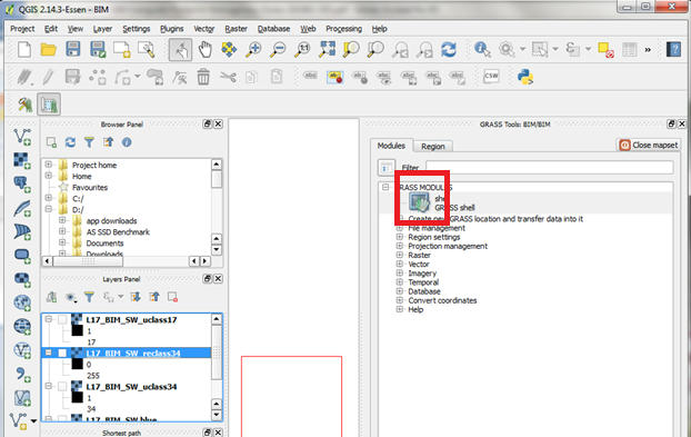
3. Import your imagery into GRASS.
a. Click on the GRASS shell icon in your GRASS tools.
b. Type in r.in.gdal to open the import window.
c. Browse to your image file and give the raster map a name, example “TBPB”. Click Run.
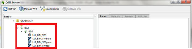
4. Start QuantumGIS Browser with GRASS.
The browser is a useful tool that enables you to easily access all the outputs we will be producing in QGIS, so that we can easily drag and drop them back into QGIS Desktop to view them again.
a. Navigate to your working directory, example “\GRASSDATA\Barbados\TBPB”. You should see a GRASS icon which represents your mapset, underneath which you should find blue, green and red bands of the imagery you imported in the previous step.
b. You may now choose to drag and drop any or all of these imagery bands into QGIS desktop to view them, but for the sake of a speedy work space, this is not yet necessary.
5. Set the region in QGIS.
a. In the GRASS shell, type g.region.
b. Under Set region to match raster map(s) select any one of the imagery bands from the dropdown list and click run.
This sets the working area to the coordinates of our imagery. (Hence why having a Geotiff is helpful") ). If you don’t have a Geotiff the coordinates can be set in the bounds tab.
). If you don’t have a Geotiff the coordinates can be set in the bounds tab.
6. Create an image group and subgroup
a. In the GRASS shell, type i.group.
b. In the Required tab, give the group a name, example “TBPB_group”.
c. In the Maps tab, select each band from the drop down list in turn, to add them to the group.
d. In the Optional tab, give the subgroup a name, example “TBPB_subgroup”.
e. Click run.
7. Perform an Unsupervised Classification.
a. In the GRASS shell, type i.cluster.
b. In the Required tab, select the group and subgroup.
c. Give the output for the signatures a name, example “TBPB_sig_11”.
d. In the Settings tab, set the initial number of classes to 11*.
*The number of classes you require for a particular image may be a matter of trial and error. The desired end result is an image where a particular range of values represent just roofs; we will discard all other values. It may be useful to create multiple signatures with different values and choose the best, example “TBPB_sig_9”, “TBPB_sig_17”, etc.
e. In the GRASS shell, type i.maxlik.
f. In the Required tab, select the group, subgroup and signature.
g. Give the raster map a name, example “TBPB_uclass_11”.
h. Click Run.
i. Grab some milk and cookies. This might take a while.
j. Repeat with other signatures if necessary.
The QGIS Browser will now come in handy. Drag and drop each classified image to QGIS Browser for viewing and comparison.
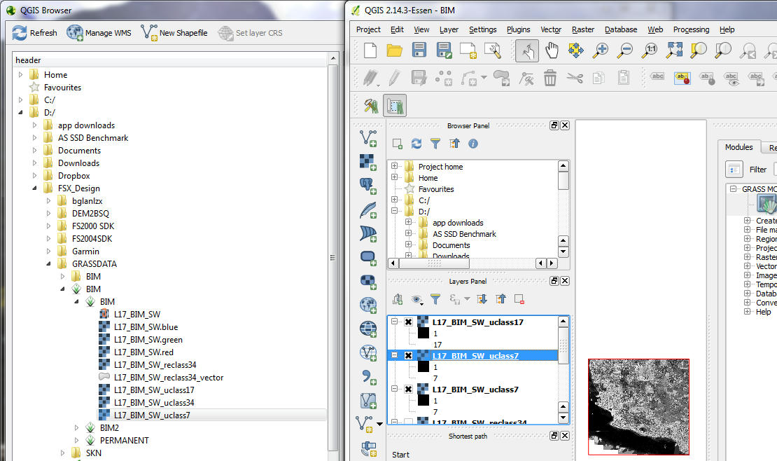
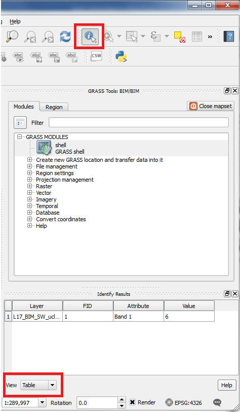
k. Check what classes represent building footprints using the Identify Features Tool. Change the View to Table. Click on an area of the classified maps to take note of what values have been applied to roofs.
For example, with 11 classes, roof values typically range from 6 to 10.
Compare different classified images to see which gives the best range of values for building footprints.
8. Reclassify the chosen raster image.
a. In the GRASS shell, type r.reclass.
b. Select your chosen classified raster map to reclassify.
c. Give the output a name, example “TBPB_reclass_11”.
d. Enter rules for the reclassification.
Example
What this does is changes all parts of the image which do not have the values which represent building footprints to black, and those that do are changed to white. These values will of course vary according to your image.
e. Click Run
We will now output the reclassified image to a BMP for post processing.
f. In the GRASS shell, type r.out.gdal.
g. Select the reclassified image.
h. Browse to a folder to save our output bitmap and give it a name, example “TBPB_reclass11.bmp”.
i. Change the raster data format to BMP. This is the necessary format for the BREC tool.
j. In the Creation Tab, check Do not write the GDAL standard colortable and select Byte as the Data Type.
k. Click Run.
l. Use the QGIS browser to load the reclassified BMP image into QGIS Desktop. It should look similar to the following.
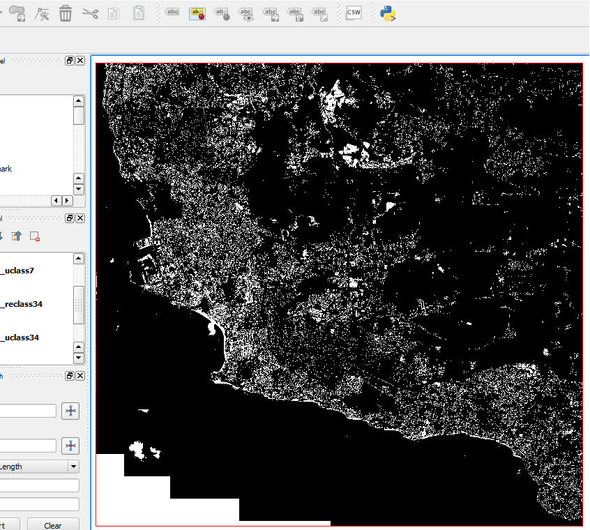
It will now be useful to remove white areas that you know are certainly not building footprints from the BMP. For example, you will notice large white areas in the bottom left corner of the above image and a few other irregularly shaped blobs, as well as most of the shoreline. This can be easily and quickly removed in your image processor of choice. I should quickly note that for production quality autogen, it will be useful to run classification on fully cleaned images which are absent of clouds and water. Use your water mask to turn all bodies of water (and especially waves which appear white) to black.
9. Use the Blob Remover Tool to clean up small specs.
a. Use CMD to open the Blob Remover tool. I found it useful to create a .bat file in notepad using similar code:
This way I can open it faster and use copy and paste from the right click menu.
b. Enter the input file name
c. Result type is set to BMP.
d. Set Blob Threshold Minimum. I use 50 on imagery which has a resolution of 1.2m/px and 100 on 0.5m/px.
e. Set Blob Threshold Maximum. I usually set to 0.
f. Grab some coffee.
g. Your output file should now be in the same directory with _br50_0.bmp at the end.
10. Import cleaned raster map and convert it to a vector shapefile.
a. Click on the GRASS shell icon, type in r.in.gdal, browse to your image file & enter the raster map name.
b. In the Optional tab check Override Projection and Force Lat/Lon Maps to fit into geographic coordinates. This will allow for import of an unrectified image.
c. Click Run.
d. Click on the GRASS shell icon, type in r.region, select the recently imported image and in the Existing tab check Set from Current region and click Run.
e. Now drag and drop the image from the QGIS Browser to the QGIS Desktop to confirm that it has been loaded and rectified correctly.
f. Click on the GRASS shell icon, type in r.to.vect.
g. Select your input map.
h. Give your output vector map a name, example “TBPB_reclass11_br_50_0_vector”
i. Set Output feature type to Area and Click Run.
j. Click on the GRASS shell icon, type in v.out.ogr.
k. Select the vector to export, provide a directory and file name, example, “TBPB_reclass11_br_50_0_vector.shp” and select ESRI_Shapefile as the Data format to write and click Run.
l. Take a sip of that coffee.
m. Drag and drop the shapefile from the Browser to QGIS Desktop for viewing.
n. Click on the Toggle Editing button and then the Select by Expression Button.
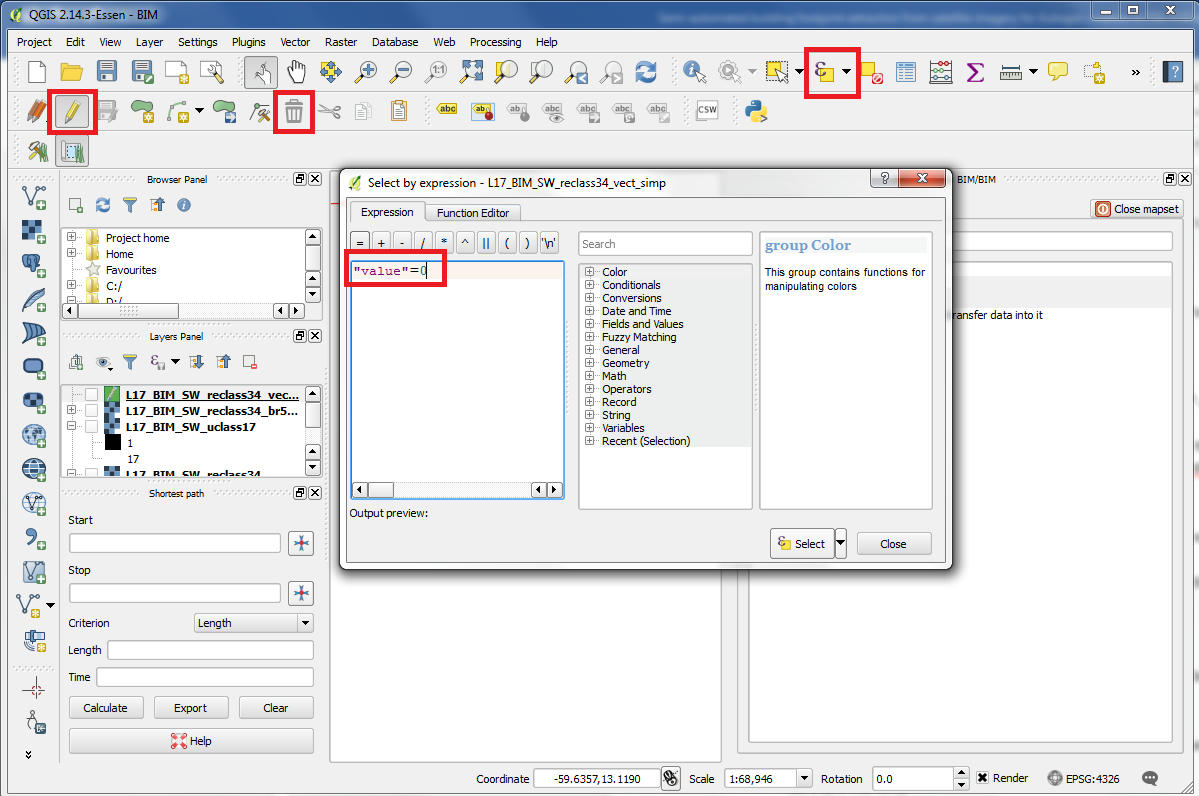
o. Enter the expression “value” = 0 or “color” = 0 to select all polygons which were black areas, then delete those polygons.
p. Go to Vector Menu > Geomtery Tools > Simplifiy Geometries…
The Default value of 0.0001 should work well. Save to a new file, example “TBPB_reclass11_br_50_0_vector_simp.shp”. Click OK.
11. Export Autogen using Scenproc.
It’s finally SCENPROC time!
Run similar code through ScenProc. FWIDTH and FLENGTH ensure that only the smaller buildings for this area are generated. You can choose to leave this out.
12. Open the corresponding area in Annotator. Now would be a good time to clean up any poorly placed/sized buildings.
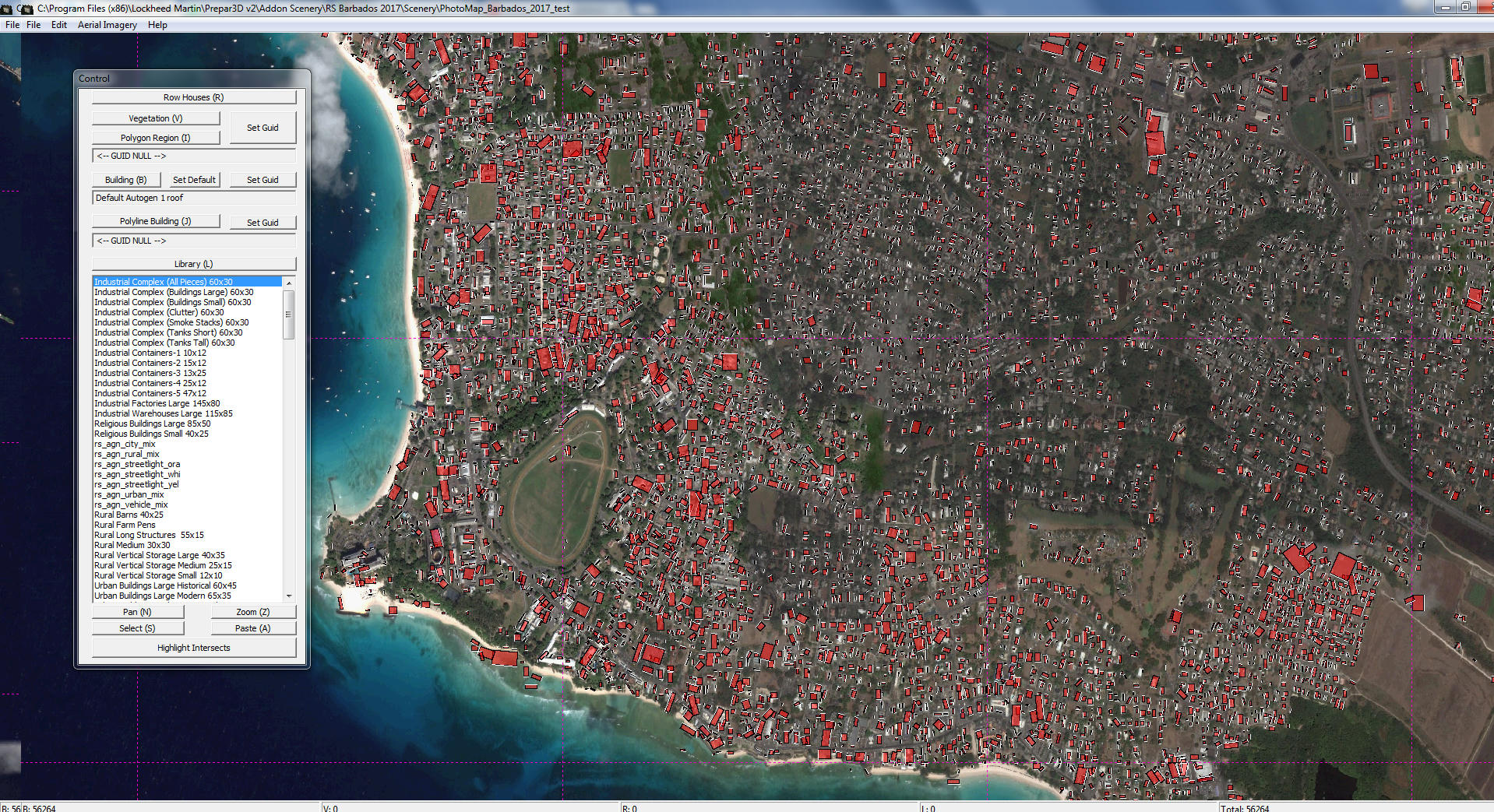
No more drawing thousands of rectangles for you!!!
13. Open your simulator and marvel at how far you could possibly take your autogen!!!
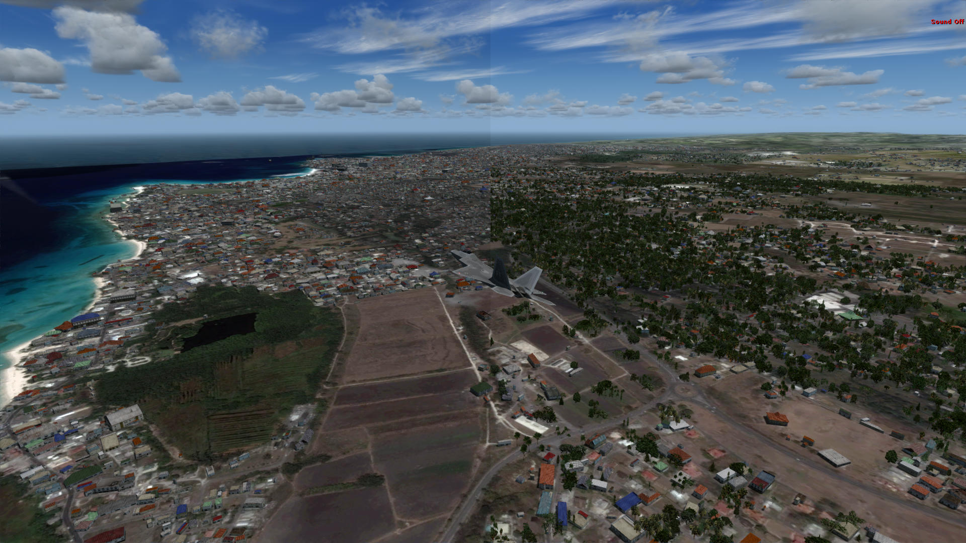
Throw in some “Fully-Automated Tree Extraction from Satellite Imagery for Autogen Creation in FSX/P3D using ScenProc” and you can hardly tell that you didn’t place those buildings manually!!!
Excuse the scientific research paper headline, but that's all I've been reading over the last few weeks!
Below I'll attempt to detail a method I have revised to semi-automatically produce autogen for FSX/P3D. Hopefully this will lead to some discussion and improvement that this entire community can benefit from. My results have been somewhat satisfactory using 2 different methods; one using free tools and the other using commercial (and rather expensive) software. Here I will outline the use of the free tools, and later, possibly produce a detailed document of every step necessary, when the results have been proven repeatable and reliable by others here.
Please note this method outlines the bare minimums to obtain barely useful results. This simplified approach is open to improvement. I am sure there are steps that I have left out that could improve results.
Tools needed:
· Quantum GIS (which comes with GRASS plugin):
https://www.qgis.org/en/site/forusers/download.html#
· BREC4GEM:
http://ftp.openquake.org/idct/brec/BREC4GEM.zip
or
http://www.mediafire.com/download/46vgk7ti3tgh3dt/BREC4GEM.zip
· Your favorite GIS software: I prefer GlobalMapper but ArcGIS and QGIS can also be used.
· Your favorite image processing software like Photoshop, Paintshop or (free) gimp.
· And last but not least the hand-dandy ScenProc by Arno.
Method:
1. Obtain satellite imagery of your desired area. Obviously.
My test area was the Southwest quarter of Barbados, west of TBPB. Nice mix of densely packed small buildings (the hardest to create autogen for), small roads, bare earth, water and vegetation. It is helpful to have your image as a geo-rectified GeoTiff.
2. Start QuantumGIS Desktop with GRASS.
a. In the Plugins Menu go to GRASS > New Mapset.
b. Create a new GRASS database directory called “GRASSDATA” in our working directory of choice.
c. Create a new location and name it, example “Barbados”.
d. Create a new mapset, example “TBPB”.
e. Click Finish. The GRASS Tools on the right of QGIS should now become available for use.
3. Import your imagery into GRASS.
a. Click on the GRASS shell icon in your GRASS tools.
b. Type in r.in.gdal to open the import window.
c. Browse to your image file and give the raster map a name, example “TBPB”. Click Run.
4. Start QuantumGIS Browser with GRASS.
The browser is a useful tool that enables you to easily access all the outputs we will be producing in QGIS, so that we can easily drag and drop them back into QGIS Desktop to view them again.
a. Navigate to your working directory, example “\GRASSDATA\Barbados\TBPB”. You should see a GRASS icon which represents your mapset, underneath which you should find blue, green and red bands of the imagery you imported in the previous step.
b. You may now choose to drag and drop any or all of these imagery bands into QGIS desktop to view them, but for the sake of a speedy work space, this is not yet necessary.
5. Set the region in QGIS.
a. In the GRASS shell, type g.region.
b. Under Set region to match raster map(s) select any one of the imagery bands from the dropdown list and click run.
This sets the working area to the coordinates of our imagery. (Hence why having a Geotiff is helpful
). If you don’t have a Geotiff the coordinates can be set in the bounds tab.6. Create an image group and subgroup
a. In the GRASS shell, type i.group.
b. In the Required tab, give the group a name, example “TBPB_group”.
c. In the Maps tab, select each band from the drop down list in turn, to add them to the group.
d. In the Optional tab, give the subgroup a name, example “TBPB_subgroup”.
e. Click run.
7. Perform an Unsupervised Classification.
a. In the GRASS shell, type i.cluster.
b. In the Required tab, select the group and subgroup.
c. Give the output for the signatures a name, example “TBPB_sig_11”.
d. In the Settings tab, set the initial number of classes to 11*.
*The number of classes you require for a particular image may be a matter of trial and error. The desired end result is an image where a particular range of values represent just roofs; we will discard all other values. It may be useful to create multiple signatures with different values and choose the best, example “TBPB_sig_9”, “TBPB_sig_17”, etc.
e. In the GRASS shell, type i.maxlik.
f. In the Required tab, select the group, subgroup and signature.
g. Give the raster map a name, example “TBPB_uclass_11”.
h. Click Run.
i. Grab some milk and cookies. This might take a while.
j. Repeat with other signatures if necessary.
The QGIS Browser will now come in handy. Drag and drop each classified image to QGIS Browser for viewing and comparison.
k. Check what classes represent building footprints using the Identify Features Tool. Change the View to Table. Click on an area of the classified maps to take note of what values have been applied to roofs.
For example, with 11 classes, roof values typically range from 6 to 10.
Compare different classified images to see which gives the best range of values for building footprints.
8. Reclassify the chosen raster image.
a. In the GRASS shell, type r.reclass.
b. Select your chosen classified raster map to reclassify.
c. Give the output a name, example “TBPB_reclass_11”.
d. Enter rules for the reclassification.
Example
Code:
0 thru 5 = 0

6 thru 10 = 255
11 = 0e. Click Run
We will now output the reclassified image to a BMP for post processing.
f. In the GRASS shell, type r.out.gdal.
g. Select the reclassified image.
h. Browse to a folder to save our output bitmap and give it a name, example “TBPB_reclass11.bmp”.
i. Change the raster data format to BMP. This is the necessary format for the BREC tool.
j. In the Creation Tab, check Do not write the GDAL standard colortable and select Byte as the Data Type.
k. Click Run.
l. Use the QGIS browser to load the reclassified BMP image into QGIS Desktop. It should look similar to the following.
It will now be useful to remove white areas that you know are certainly not building footprints from the BMP. For example, you will notice large white areas in the bottom left corner of the above image and a few other irregularly shaped blobs, as well as most of the shoreline. This can be easily and quickly removed in your image processor of choice. I should quickly note that for production quality autogen, it will be useful to run classification on fully cleaned images which are absent of clouds and water. Use your water mask to turn all bodies of water (and especially waves which appear white) to black.
9. Use the Blob Remover Tool to clean up small specs.
a. Use CMD to open the Blob Remover tool. I found it useful to create a .bat file in notepad using similar code:
Code:
START cmd.exe /k "D:\Program Files\BREC\BlobRemover\blob_removerwin.exe"b. Enter the input file name
c. Result type is set to BMP.
d. Set Blob Threshold Minimum. I use 50 on imagery which has a resolution of 1.2m/px and 100 on 0.5m/px.
e. Set Blob Threshold Maximum. I usually set to 0.
f. Grab some coffee.
g. Your output file should now be in the same directory with _br50_0.bmp at the end.
10. Import cleaned raster map and convert it to a vector shapefile.
a. Click on the GRASS shell icon, type in r.in.gdal, browse to your image file & enter the raster map name.
b. In the Optional tab check Override Projection and Force Lat/Lon Maps to fit into geographic coordinates. This will allow for import of an unrectified image.
c. Click Run.
d. Click on the GRASS shell icon, type in r.region, select the recently imported image and in the Existing tab check Set from Current region and click Run.
e. Now drag and drop the image from the QGIS Browser to the QGIS Desktop to confirm that it has been loaded and rectified correctly.
f. Click on the GRASS shell icon, type in r.to.vect.
g. Select your input map.
h. Give your output vector map a name, example “TBPB_reclass11_br_50_0_vector”
i. Set Output feature type to Area and Click Run.
j. Click on the GRASS shell icon, type in v.out.ogr.
k. Select the vector to export, provide a directory and file name, example, “TBPB_reclass11_br_50_0_vector.shp” and select ESRI_Shapefile as the Data format to write and click Run.
l. Take a sip of that coffee.
m. Drag and drop the shapefile from the Browser to QGIS Desktop for viewing.
n. Click on the Toggle Editing button and then the Select by Expression Button.
o. Enter the expression “value” = 0 or “color” = 0 to select all polygons which were black areas, then delete those polygons.
p. Go to Vector Menu > Geomtery Tools > Simplifiy Geometries…
The Default value of 0.0001 should work well. Save to a new file, example “TBPB_reclass11_br_50_0_vector_simp.shp”. Click OK.
11. Export Autogen using Scenproc.
It’s finally SCENPROC time!
Run similar code through ScenProc. FWIDTH and FLENGTH ensure that only the smaller buildings for this area are generated. You can choose to leave this out.
Code:
#Barbados 2017 autogen


ImportOGR|D:\GRASSDATA\TBPB_reclass11_br_50_0_vector_simp.shp |*|*|NOREPROJ
SplitGrid|AGN|*
SETAGNBUILDINGHEIGHT|*|1.0;0.0;0.0;0.0
CREATEAGNGENBUILD|FTYPE=*;*;FWIDTH<50;FLENGTH<50|{2e39baf8-699f-4055-931c-992a64c0e206}

EXPORTAGN|P3D v2| C:\Program Files (x86)\Lockheed Martin\Prepar3D v2\Addon Scenery\RS Barbados 2017\Texture
12. Open the corresponding area in Annotator. Now would be a good time to clean up any poorly placed/sized buildings.
No more drawing thousands of rectangles for you!!!
13. Open your simulator and marvel at how far you could possibly take your autogen!!!
Throw in some “Fully-Automated Tree Extraction from Satellite Imagery for Autogen Creation in FSX/P3D using ScenProc” and you can hardly tell that you didn’t place those buildings manually!!!


